PDF Publication Title:
Text from PDF Page: 004
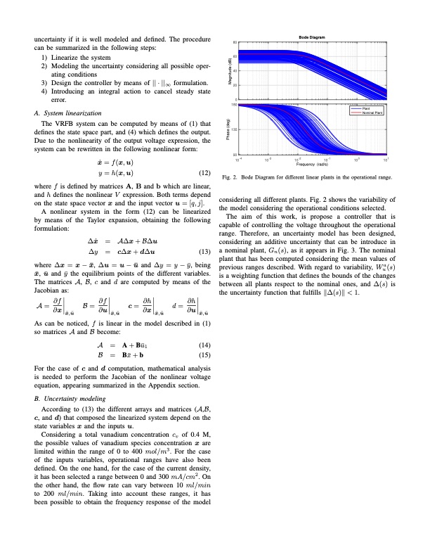
uncertainty if it is well modeled and defined. The procedure can be summarized in the following steps: 1) Linearize the system 2) Modeling the uncertainty considering all possible oper- ating conditions 3) Design the controller by means of || · ||∞ formulation. 4) Introducing an integral action to cancel steady state error. A. System linearization The VRFB system can be computed by means of (1) that defines the state space part, and (4) which defines the output. Due to the nonlinearity of the output voltage expression, the system can be rewritten in the following nonlinear form: x ̇ = f ( x , u ) y = h(x, u) (12) where f is defined by matrices A, B and b which are linear, and h defines the nonlinear V expression. Both terms depend on the state space vector x and the input vector u = [q, j]. A nonlinear system in the form (12) can be linearized by means of the Taylor expansion, obtaining the following formulation: Bode Diagram ∆x ̇ = A∆x+B∆u ∆y = c∆x + d∆u (13) Fig. 2. Bode Diagram for different linear plants in the operational range. considering all different plants. Fig. 2 shows the variability of the model considering the operational conditions selected. The aim of this work, is propose a controller that is capable of controlling the voltage throughout the operational range. Therefore, an uncertainty model has been designed, considering an additive uncertainty that can be introduce in a nominal plant, Gn(s), as it appears in Fig. 3. The nominal plant that has been computed considering the mean values of previous ranges described. With regard to variability, Wua(s) is a weighting function that defines the bounds of the changes between all plants respect to the nominal ones, and ∆(s) is the uncertainty function that fulfills ∥∆(s)∥ < 1. where ∆x = x−x ̄, ∆u = u−u ̄ and ∆y = y−y ̄, being x ̄, u ̄ and y ̄ the equilibrium points of the different variables. The matrices A, B, c and d are computed by means of the Jacobian as: A= ∂f B= ∂f c= ∂h d= ∂h ∂x x ̄,u ̄ ∂u x ̄,u ̄ ∂x x ̄,u ̄ ∂u x ̄,u ̄ As can be noticed, f is linear in the model described in (1) so matrices A and B become: A = A + Bu ̄1 B = Bx ̄+b (14) (15) For the case of c and d computation, mathematical analysis is needed to perform the Jacobian of the nonlinear voltage equation, appearing summarized in the Appendix section. B. Uncertainty modeling According to (13) the different arrays and matrices (A,B, c, and d) that composed the linearized system depend on the state variables x and the inputs u. Considering a total vanadium concentration cv of 0.4 M, the possible values of vanadium species concentration x are limited within the range of 0 to 400 mol/m3. For the case of the inputs variables, operational ranges have also been defined. On the one hand, for the case of the current density, it has been selected a range between 0 and 300 mA/cm2. On the other hand, the flow rate can vary between 10 ml/min to 200 ml/min. Taking into account these ranges, it has been possible to obtain the frequency response of the model 80 60 40 20 0 180 135 90 10-4 10-3 Plant Nominal Plant Phase (deg) Magnitude (dB) 10-2 10-1 100 Frequency (rad/s) 101PDF Image | H control of a redox flow battery overpotentials
PDF Search Title:
H control of a redox flow battery overpotentialsOriginal File Name Searched:
2523-Flow-controlling-tuning-for-the-voltage-flow-battery.pdfDIY PDF Search: Google It | Yahoo | Bing
Salgenx Redox Flow Battery Technology: Salt water flow battery technology with low cost and great energy density that can be used for power storage and thermal storage. Let us de-risk your production using our license. Our aqueous flow battery is less cost than Tesla Megapack and available faster. Redox flow battery. No membrane needed like with Vanadium, or Bromine. Salgenx flow battery
| CONTACT TEL: 608-238-6001 Email: greg@salgenx.com | RSS | AMP |