PDF Publication Title:
Text from PDF Page: 017
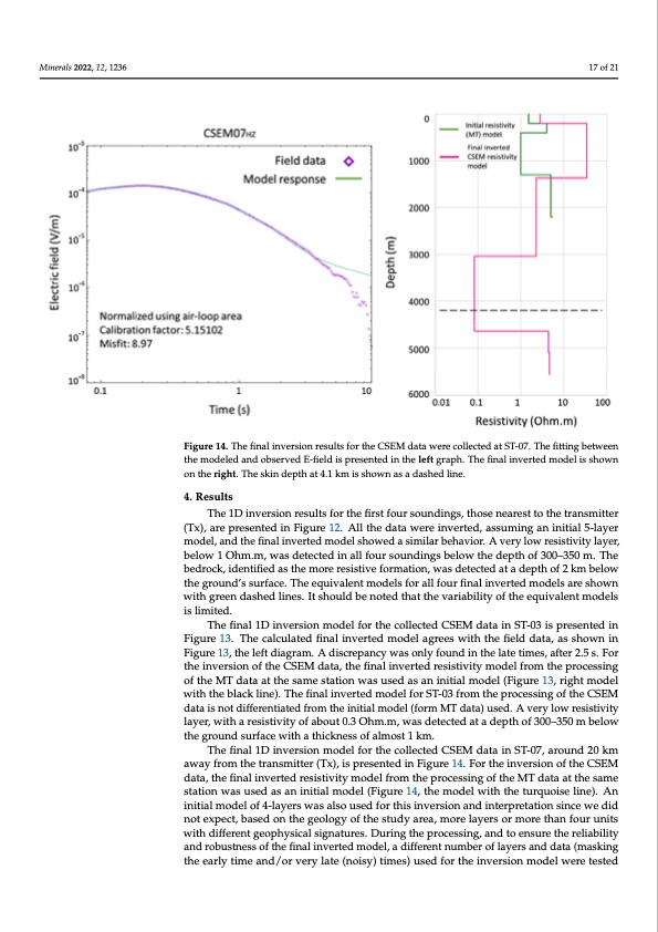
and robustness of the final inverted model, a different number of layers and data (masking Minerals 2022, 12, 1236 the early time and/or very late (noisy) times) used for the inversion model were tested and evaluated. The final inverted model for ST-07, 20 km away from Tx, is presented in Figure 14 (model on the right). The calculated misfit is 8.97. Based on the resulting final resistivity model, after the depth of 1.3 km, the resistivity reached 3.1 Ohm.m and a very low resis- 17 of 21 tivity layer, with a resistivity of about 0.1 Ohm.m, was detected at a depth of 3 km below the ground surface. Figure 14. The final inversion results for the CSEM data were collected at ST-07. The fitting between Figure 14. The final inversion results for the CSEM data were collected at ST-07. The fitting between the modeled and observed E-field is presented in the left graph. The final inverted model is shown the modeled and observed E-field is presented in the left graph. The final inverted model is shown ontherightt..Thesskiindeptthatt4..1Kkm is shown as a dashed line. 4. Results The final 2D inversion model using the REBOCC code for the SW–NE profile, com- posed of the ST-01 to ST-04, is shown in Figure 15. It is quite risky to apply 2D inversion The 1D inversion results for the first four soundings, those nearest to the transmitter (Tx), are presented in Figure 12. All the data were inverted, assuming an initial 5-layer on only four soundings, but we decided to do so to compare the final tomogra phic image with the final 1D inverted models, as presented in Figure 12. A very low resistivity anom- model, and the final inverted model showed a similar behavior. A very low resistivity layer, aly with a resistivity of 0.3 Ohm.m was detected at a depth of 350 m below the ground below 1 Ohm.m, was detected in all four soundings below the depth of 300–350 m. The surface. This finding is in agreement with the 1D models in Figure 12. This very conduc- bedrock, identified as the more resistive formation, was detected at a depth of 2 km below the ground’s surface. The equivalent models for all four final inverted models are shown tive zone seems to extend below the maximum depth of the model, that is, 1 Km. with green dashed lines. It should be noted that the variability of the equivalent models is limited. The final 1D inversion model for the collected CSEM data in ST-03 is presented in Figure 13. The calculated final inverted model agrees with the field data, as shown in Figure 13, the left diagram. A discrepancy was only found in the late times, after 2.5 s. For the inversion of the CSEM data, the final inverted resistivity model from the processing of the MT data at the same station was used as an initial model (Figure 13, right model with the black line). The final inverted model for ST-03 from the processing of the CSEM data is not differentiated from the initial model (form MT data) used. A very low resistivity layer, with a resistivity of about 0.3 Ohm.m, was detected at a depth of 300–350 m below the ground surface with a thickness of almost 1 km. The final 1D inversion model for the collected CSEM data in ST-07, around 20 km away from the transmitter (Tx), is presented in Figure 14. For the inversion of the CSEM data, the final inverted resistivity model from the processing of the MT data at the same station was used as an initial model (Figure 14, the model with the turquoise line). An initial model of 4-layers was also used for this inversion and interpretation since we did not expect, based on the geology of the study area, more layers or more than four units with different geophysical signatures. During the processing, and to ensure the reliability and robustness of the final inverted model, a different number of layers and data (masking the early time and/or very late (noisy) times) used for the inversion model were testedPDF Image | First High-Power CSEM
PDF Search Title:
First High-Power CSEMOriginal File Name Searched:
minerals-12-01236-v2.pdfDIY PDF Search: Google It | Yahoo | Bing
Product and Development Focus for Infinity Turbine
ORC Waste Heat Turbine and ORC System Build Plans: All turbine plans are $10,000 each. This allows you to build a system and then consider licensing for production after you have completed and tested a unit.Redox Flow Battery Technology: With the advent of the new USA tax credits for producing and selling batteries ($35/kW) we are focussing on a simple flow battery using shipping containers as the modular electrolyte storage units with tax credits up to $140,000 per system. Our main focus is on the salt battery. This battery can be used for both thermal and electrical storage applications. We call it the Cogeneration Battery or Cogen Battery. One project is converting salt (brine) based water conditioners to simultaneously produce power. In addition, there are many opportunities to extract Lithium from brine (salt lakes, groundwater, and producer water).Salt water or brine are huge sources for lithium. Most of the worlds lithium is acquired from a brine source. It's even in seawater in a low concentration. Brine is also a byproduct of huge powerplants, which can now use that as an electrolyte and a huge flow battery (which allows storage at the source).We welcome any business and equipment inquiries, as well as licensing our turbines for manufacturing.| CONTACT TEL: 608-238-6001 Email: greg@infinityturbine.com | RSS | AMP |