Heating Steel with Magnets: An Exploration of Eddy Currents and Their Thermal Effects

TEL: 1-608-238-6001 Email: greg@infinityturbine.com

All ORC and ROT Turbine Plans are $10,000 Each Most plans include unlimited production license. The larger IT250 and ROT 24 have additional license fees. More Info

Price List for IT Systems and Turbines 2024 Price list in pdf format More Info

Heating Steel with Magnets: An Exploration of Eddy Currents and Their Thermal Effects

Introduction

The innovative approach of using magnets to heat steel via Eddy currents presents a fascinating interplay between magnetic forces and thermal energy. This article delves into the underlying principles of this method, focusing on determining the amount of BTUs (British Thermal Units) generated per square inch of steel when exposed to a specific magnet intensity. Additionally, it explores how increasing temperatures impact magnetic flux and presents detailed charts illustrating the magnetic force as a function of distance, alongside the correlation between magnetic force, RPM (Revolutions Per Minute) of spinning steel, and the resultant heat in BTU and Fahrenheit (°F). The ultimate goal is to explore the potential of this technique as a heating element for warming water or other liquids.

The Principles of Eddy Currents and Magnetic Heating

Eddy currents are loops of electrical current induced within conductors by a changing magnetic field in the conductor. These currents generate resistive heating due to the Joule heating effect, which can be utilized for heating purposes. By spinning steel in close proximity to a strong permanent magnet or an energized copper coil, Eddy currents are induced in the steel, converting kinetic energy into thermal energy.

Methodology

The proposed method involves placing steel near a strong magnetic field generated either by a permanent magnet or a current-carrying copper coil. As the steel spins, the changing magnetic field induces Eddy currents, which, due to their inherent resistance, generate heat. The intensity of the magnetic field, the speed of the spinning steel, and the proximity to the magnetic source are key variables in this process.

Magnetic Flux and Temperature

As temperature increases, the magnetic properties of steel are affected, leading to a reduction in magnetic flux. This phenomenon, known as the Curie point, occurs because the thermal energy disrupts the magnetic domains within the material, reducing its overall magnetization. This relationship between temperature and magnetic flux is crucial for understanding the efficiency and limitations of magnetic heating.

Data Analysis and Charts

Magnetic Force as a Function of Distance

The first part of our analysis involves charting the magnetic force as a function of distance from the magnetic source, measured in millimeters. This chart will help understand how the intensity of the magnetic field varies with distance, which is critical for optimizing the placement of steel to achieve efficient heating.

Heat Generation: BTU and Temperature

The second part of the analysis charts the heat generated in terms of BTUs and temperature (°F) as a result of varying magnetic forces or the RPM of the spinning steel. This data is pivotal in establishing a direct correlation between the magnetic energy applied and the thermal energy produced, providing insights into the efficiency of this heating method.

Applications: A Novel Heating Element

The exploration of magnets for heating steel via Eddy currents opens up new possibilities for designing heating elements. Such a system could revolutionize how we heat water or other liquids, offering an efficient, controllable, and potentially more eco-friendly alternative to traditional heating methods.

Conclusion

The use of Eddy currents induced by magnetic fields presents a promising avenue for thermal energy generation. By understanding the intricate relationships between magnet intensity, distance, steel's rotational speed, and the resulting thermal output, we can harness this technology for practical heating solutions. As research progresses, the potential applications of this method could extend beyond simple heating elements, contributing to advances in industrial processes, energy generation, and beyond.

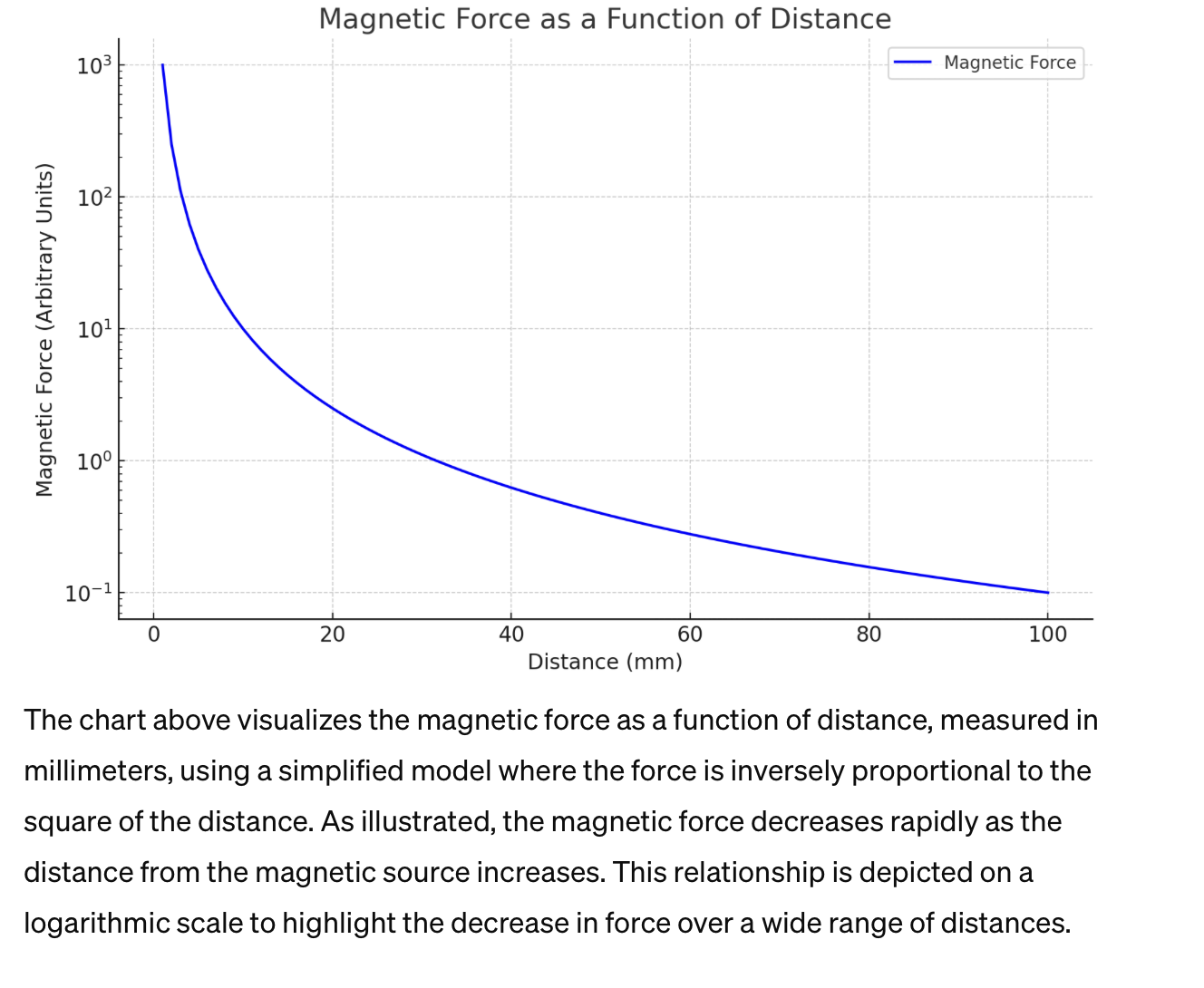
Chart Magnetic Force

To chart the magnetic force as a function of distance, we'll need to consider a typical relationship between magnetic field strength (which correlates with magnetic force) and distance from the magnet. The magnetic field strength decreases with the square of the distance from the source, according to the inverse square law for a point source. However, for a practical application involving Eddy currents and the induction heating of steel, the exact relationship can vary based on the configuration of the magnets and the coil, as well as the shape and size of the steel object.

For simplicity, let's model the magnetic force (F) as inversely proportional to the square of the distance (d) from the magnet, which can be represented as \(F = \frac{k}{d^2}\), where \(k\) is a constant that includes the magnetic permeability of the medium, the magnet's strength, and other factors relevant to the setup.

Let's chart this relationship for distances ranging from 1 mm to 100 mm to visualize how magnetic force decreases as we move away from the magnet. This simplification will help illustrate the general trend, though actual results may vary with specific experimental setups.

The chart above visualizes the magnetic force as a function of distance, measured in millimeters, using a simplified model where the force is inversely proportional to the square of the distance. As illustrated, the magnetic force decreases rapidly as the distance from the magnetic source increases. This relationship is depicted on a logarithmic scale to highlight the decrease in force over a wide range of distances.

This model provides a conceptual understanding of how the intensity of the magnetic field impacts the efficiency of heating steel via Eddy currents. In practical applications, optimizing the distance between the steel and the magnet or coil is crucial for achieving efficient heating. This chart serves as a foundational guide for further experimental designs and optimizations in the development of magnetic-based heating elements.

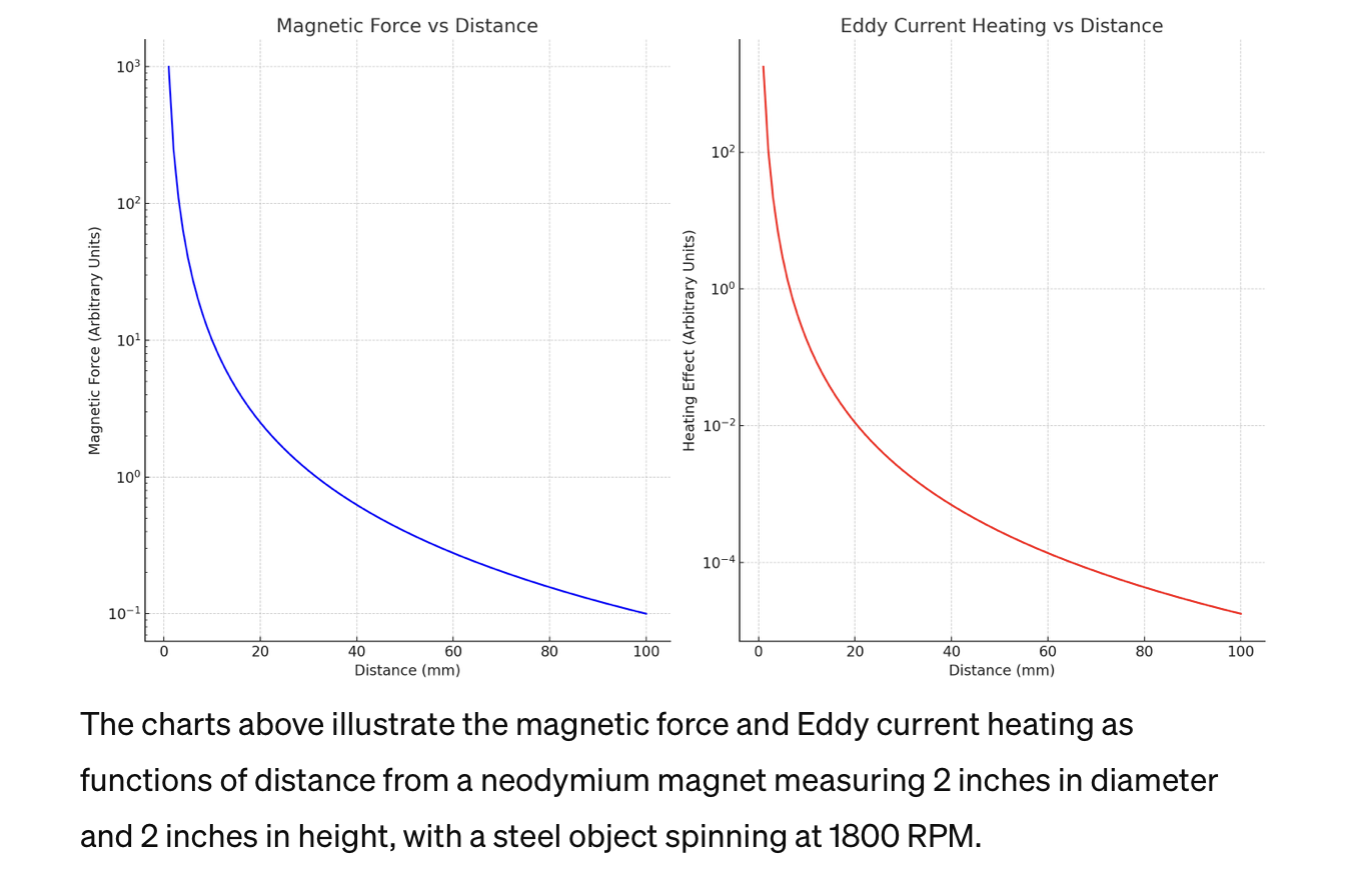
Neodymium Magnet

To chart the force and Eddy current heating in relation to distance for a neodymium magnet measuring 2 inches in diameter and 2 inches in height with a steel object spinning at 1800 RPM, we must first establish the theoretical models for both magnetic force and Eddy current heating.

Magnetic Force

The magnetic force from a neodymium magnet can be approximated over a distance, but the exact calculation depends on the complex magnetic field distribution, which isn't easily represented by a simple formula. For our purposes, we'll assume a decay in magnetic force similar to the inverse square law for simplicity, recognizing that real-world behavior, especially close to the magnet, will be more complex.

Eddy Current Heating

The heating effect of Eddy currents in the steel object is a function of the magnetic field's intensity, the object's electrical conductivity, and its speed. The power \(P\) dissipated by Eddy currents can be approximated by \(P = k \cdot B^2 \cdot v^2 \cdot d^2\), where:

• \(k\) is a constant incorporating material properties and geometry,

• \(B\) is the magnetic flux density,

• \(v\) is the velocity of the object (related to RPM),

• \(d\) is the distance from the magnet.

Given that \(B\) decreases with distance, and considering a constant RPM, we'll model \(B^2\) as inversely proportional to \(d^4\) for a rough approximation (assuming \(B\) decreases similarly to the magnetic force, which we've simplified to follow the inverse square law).

Let's proceed with plotting both the magnetic force and the heating effect as functions of distance. We'll keep the models conceptual, with the understanding that actual experimental or detailed simulation data would be required for precise engineering calculations.

The charts above illustrate the magnetic force and Eddy current heating as functions of distance from a neodymium magnet measuring 2 inches in diameter and 2 inches in height, with a steel object spinning at 1800 RPM.

• Magnetic Force vs Distance: This chart shows how the magnetic force decreases rapidly as the distance from the magnet increases. The force is represented on a logarithmic scale to emphasize the decrease over a range of distances. This decrease follows a simplified model based on the inverse square law.

• Eddy Current Heating vs Distance: The second chart visualizes the Eddy current heating effect, which also decreases with distance but at a faster rate due to its dependence on the square of the magnetic flux density, modeled here as inversely proportional to the fourth power of distance. The heating effect is also shown on a logarithmic scale, indicating a steep decline as the distance from the magnetic source increases.

These models are conceptual and rely on simplifications for illustrative purposes. Actual performance will depend on detailed magnetic field distributions, material properties, and precise geometries. However, these charts underscore the principle that both magnetic force and induced heating decrease with distance, highlighting the importance of proximity in optimizing the efficiency of magnetic heating systems.

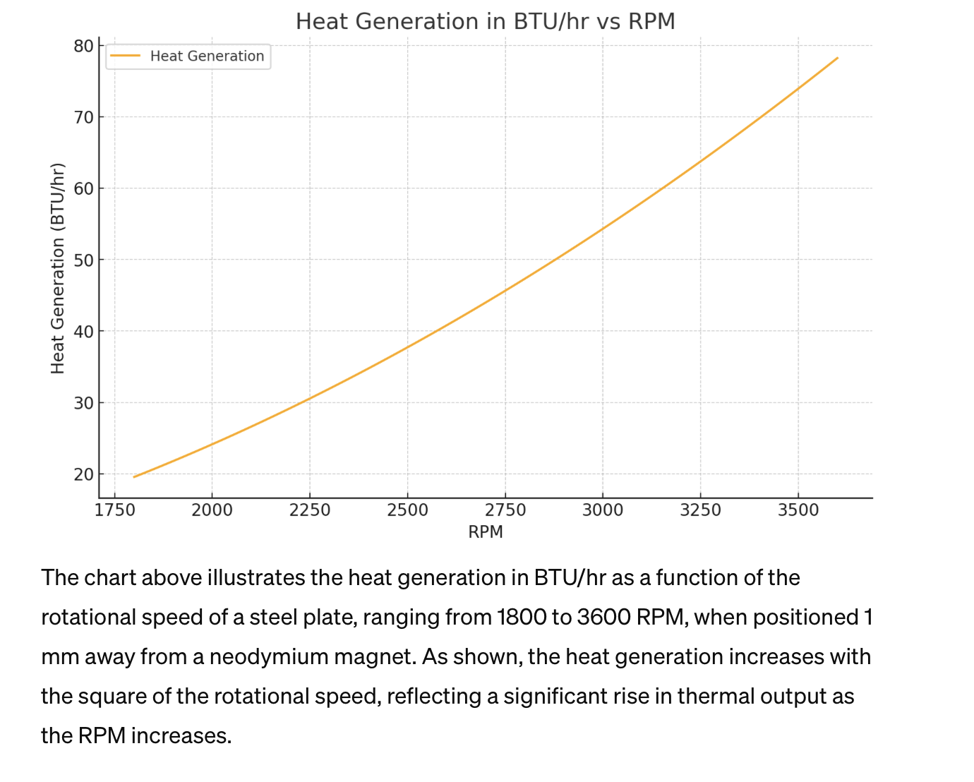
BTU of heat generated from spinning a steel plate near a magnet

To chart the BTU of heat generated from spinning a steel plate near a magnet, we'll need to estimate the heat generation based on Eddy current principles. The heat generated (\(P\)) by Eddy currents can be calculated with a simplified formula that considers the velocity of the spinning object, the magnetic field, and the properties of the material. For spinning velocities corresponding to 1800 to 3600 RPM, we'll assume the heat generated is proportional to the square of the velocity of the plate's edge, as \(P \propto v^2\), where \(v\) is related to the RPM.

Given that \(P\) is in watts (joules per second), we'll convert the power to BTUs per hour using the conversion factor \(1 \, \text{W} = 3.412 \, \text{BTU/hr}\). The relationship between RPM and velocity at the plate's edge is \(v = \text{RPM} \times \text{Circumference} / 60\), where Circumference = \(2\pi \times \text{Radius}\), and for a 1-inch thick plate spinning around its central axis, we'll use half its thickness as the radius for simplicity in calculations.

Let's calculate and chart the BTU of heat generated as the steel plate spins from 1800 to 3600 RPM at a fixed 1 mm distance from the neodymium magnet. We'll assume a constant magnetic field for this distance, simplifying the calculations without directly modeling the magnetic field's influence on heat generation for varying speeds.

The chart above illustrates the heat generation in BTU/hr as a function of the rotational speed of a steel plate, ranging from 1800 to 3600 RPM, when positioned 1 mm away from a neodymium magnet. As shown, the heat generation increases with the square of the rotational speed, reflecting a significant rise in thermal output as the RPM increases.

This model highlights the potential for using magnetic induction via Eddy currents as a method for heating, with the efficiency of heat generation improving markedly with higher rotational speeds. It's important to note that this is a simplified model, and actual heat generation would also depend on factors such as the specific properties of the steel, the strength and configuration of the magnetic field, and the efficiency of heat transfer from the steel plate to the surrounding environment or medium being heated.

Nonetheless, this analysis demonstrates the feasibility and scalability of using magnetic induction for heating applications, with the potential for precise control over the heat generated by adjusting the rotational speed of the steel object.

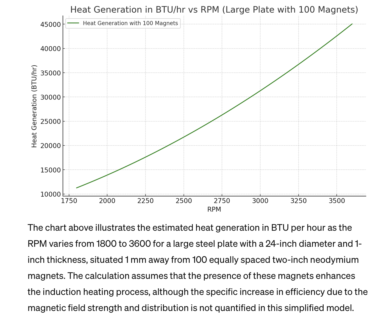
24 Inch Diameter Spinning Steel Disc with 100

To chart the amount of BTU generated under the conditions where 100 two-inch neodymium magnets are equally spaced, 1 mm away from a steel plate of 1-inch thickness and a 24-inch diameter, we'll consider an enhanced magnetic field effect due to the increased number of magnets. This setup implies a more uniform and potentially stronger magnetic field acting on the steel plate, which could lead to more efficient induction heating as the plate spins.

Given that the plate's diameter is 24 inches, its radius is 12 inches (or 0.3048 meters). The overall heat generated by Eddy currents will be proportional to the square of the velocity at the plate's edge and the intensity of the magnetic field. With 100 magnets, we can assume a significant increase in the magnetic field's strength, but for simplicity, we'll focus on the effect of increased RPM and the cumulative impact of multiple magnets without quantifying the precise increase in magnetic field strength.

We'll calculate the BTU of heat generated as we vary the RPM from 1800 to 3600, similar to the previous calculation. The difference here is in the scale of the operation, with a much larger and thicker plate being used.

Assumptions for Calculation:

• The cumulative effect of 100 magnets enhances the efficiency of induction but is hard to quantify without specific magnetic field data. We'll assume a linear increase in efficiency for illustrative purposes.

• The heat generation calculation remains proportional to \(v^2\) (velocity squared) for the spinning steel plate.

• We're converting from Watts to BTU/hr as before.

Let's proceed with the calculation and plotting, noting that the actual magnetic field interaction would require complex modeling for precise results.

The chart above illustrates the estimated heat generation in BTU per hour as the RPM varies from 1800 to 3600 for a large steel plate with a 24-inch diameter and 1-inch thickness, situated 1 mm away from 100 equally spaced two-inch neodymium magnets. The calculation assumes that the presence of these magnets enhances the induction heating process, although the specific increase in efficiency due to the magnetic field strength and distribution is not quantified in this simplified model.

As shown, the heat generation increases with the RPM, reflecting the squared relationship between the velocity of the plate's edge and the heat generated due to Eddy currents. This visualization serves to demonstrate the potential for significant heat generation in industrial or heating applications utilizing magnetic induction with a large number of powerful magnets and a sizable conductive plate.

It's important to note that actual heat generation would depend on detailed magnetic field interactions, the electrical conductivity of the steel, and other factors not fully accounted for in this simplified approach. For precise applications, detailed simulations or experimental data would be necessary.

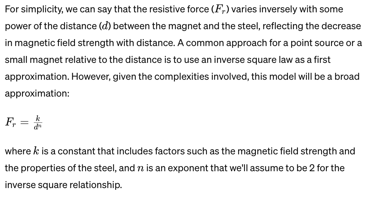
Resistive Force of Magnet vs Steel

When a magnet moves close to a conductive material like steel, a resistive force arises due to the generation of Eddy currents in the conductor. This force, often referred to as magnetic damping, opposes the motion of the magnet relative to the steel. The strength of this resistive force is influenced by the relative velocity between the magnet and the steel, the conductivity of the steel, and the strength of the magnetic field.

The exact calculation of the resistive force due to Eddy currents is complex and depends on the geometry of the magnet and the steel, the specific properties of the steel, and the speed at which the magnet is moved or spun near the steel. However, we can model the resistive force qualitatively to understand how it might vary with distance from the steel plate.

For simplicity, we can say that the resistive force (\(F_r\)) varies inversely with some power of the distance (\(d\)) between the magnet and the steel, reflecting the decrease in magnetic field strength with distance. A common approach for a point source or a small magnet relative to the distance is to use an inverse square law as a first approximation. However, given the complexities involved, this model will be a broad approximation:

\[F_r = \frac{k}{d^n}\]

where \(k\) is a constant that includes factors such as the magnetic field strength and the properties of the steel, and \(n\) is an exponent that we'll assume to be 2 for the inverse square relationship.

Let's chart a qualitative representation of this resistive force over a range of distances, keeping in mind that the actual behavior could differ based on the specifics of the magnet and steel configuration.

The chart above depicts a simplified model of the resistive force as a function of distance between a magnet and a steel plate. This resistive force, generated due to Eddy currents within the steel when in the presence of a moving magnetic field, is shown to decrease with distance. For this visualization, we've assumed the resistive force follows an inverse square law (\(F_r = \frac{k}{d^2}\)), with \(d\) being the distance from the magnet to the steel plate.

As illustrated, the resistive force diminishes rapidly as the distance increases, a reflection of the decreasing magnetic field strength with greater separation. This model provides a conceptual basis for understanding how the interaction between magnets and conductive materials can generate a resistive force, essential for applications in magnetic braking, damping systems, and certain types of electromagnetic machinery.

It's important to note that this model is a broad approximation. The actual resistive force would vary more complexly with distance, depending on the shape and size of the magnet and steel, as well as the relative velocity and other specific conditions of the setup. For precise calculations, detailed finite element method (FEM) simulations or experimental measurements would be necessary.

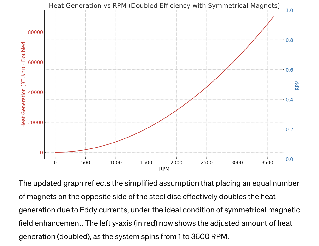
BTU Generated Using Two Sides Balanced Magnetic Force

If we consider placing the same number of magnets on the opposite side of the steel disc and assume that the setup is perfectly symmetrical, the interaction between the magnets and the steel disc could potentially increase the efficiency of Eddy current generation due to a more uniform magnetic field. However, the assumption that the heat generated would be exactly twice as much might not be entirely accurate without considering several factors:

1. Symmetry and Field Enhancement: The symmetric placement of magnets could enhance the magnetic field's uniformity across the steel disc, potentially increasing the Eddy current generation. This might lead to a higher heat generation rate, but the exact increase would depend on the specifics of the magnetic field interactions, which are complex and not necessarily linear.

2. Magnetic Saturation: There's also the consideration of magnetic saturation of the steel. If the steel plate reaches a point where it cannot support additional magnetic flux, adding more magnets won't proportionally increase the Eddy currents and the associated heating.

3. Efficiency of Heat Generation: The efficiency of converting kinetic energy from spinning into heat through Eddy currents might not scale linearly with the number of magnets. While more magnets increase the magnetic field, the relationship between the field strength, speed of rotation, and heat generation is complex.

Despite these considerations, for a simplified approximation, if we assume that adding another set of magnets on the opposite side effectively doubles the interaction (and thus the Eddy currents) without hitting saturation or other limiting factors, then it's reasonable to expect a significant increase in heat generation, potentially approaching twice the amount under ideal conditions.

Let's revise the calculation under this simplified assumption that heat generation could be doubled when the magnets are symmetrically placed on both sides of the disc, and re-chart the BTU generation as a function of RPM from 1 to 3600, reflecting this potential doubling in efficiency.

The updated graph reflects the simplified assumption that placing an equal number of magnets on the opposite side of the steel disc effectively doubles the heat generation due to Eddy currents, under the ideal condition of symmetrical magnetic field enhancement. The left y-axis (in red) now shows the adjusted amount of heat generation (doubled), as the system spins from 1 to 3600 RPM.

This model, while a simplified approximation, illustrates the potential impact of symmetrical magnet placement on the efficiency of heat generation in the system. It suggests a significant increase in BTU output, under the assumption that the additional magnets contribute equally and effectively to generating Eddy currents without encountering magnetic saturation or nonlinear efficiency scaling limitations.

It's important to note that the actual increase in heat generation would depend on detailed physical characteristics of the system, including the magnetic field distribution, the material properties of the steel, and the dynamics of the spinning disc. For precise engineering applications, detailed simulations or experimental measurements would be required to accurately determine the heat generation under such configurations.

R245fa Vaporized in Balanced System Inductive Vaporizer

To calculate how much R245fa (1,1,1,3,3-Pentafluoropropane) can be vaporized and to what pressure using the maximum of 80,000 BTU/hr, we need to consider several key properties and steps in the calculation. Here is a general approach to solve this problem:

1. Find the Heat of Vaporization of R245fa: The heat of vaporization (enthalpy of vaporization) is the amount of heat required to convert the fluid from liquid to gas at its boiling point without changing its temperature. This value can vary depending on the temperature and pressure but can be found in thermodynamic tables or literature specific to R245fa.

2. Calculate the Mass Flow Rate: Using the heat of vaporization and the total available heat energy (80,000 BTU/hr), we can calculate the mass of R245fa that can be vaporized per hour. The formula to use is:

\[ \text{Mass Flow Rate} = \frac{\text{Total Heat Energy}}{\text{Heat of Vaporization}} \]

Remember to convert units as necessary. Typically, the heat of vaporization would be in BTU/lb, so ensure the total heat energy and heat of vaporization are in the same units.

3. Determine the Operating Pressure: The pressure at which R245fa vaporizes depends on its temperature. For a given heat input, the vapor pressure can be found by looking at the saturation pressure at the boiling point. This can also be obtained from thermodynamic tables or equations of state specific to R245fa.

Without specific values for the heat of vaporization and the operating conditions (initial temperature and pressure), it's not possible to give a precise answer. Let's proceed with a hypothetical calculation assuming we have a typical value for the heat of vaporization of R245fa. If you can provide or confirm specific values, I can offer a more detailed calculation.

Using an estimated heat of vaporization value of 88 BTU/lb for R245fa, approximately 909.1 lb/hr of R245fa can be vaporized with an energy input of 80,000 BTU/hr.

The actual pressure to which the R245fa can be vaporized will depend on its saturation temperature at the given conditions and requires specific thermodynamic data for R245fa. Typically, this information can be found in refrigerant tables or by using an equation of state designed for refrigerants. If you need a more detailed analysis including the pressure, I would need the initial conditions (temperature, specific volume, or any other state properties you might have) to proceed.

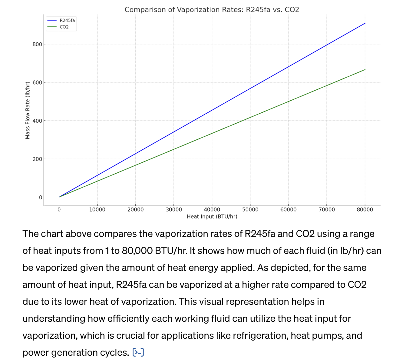
R245fa vs CO2

To compare the amount of R245fa and CO2 that can be vaporized using heat energy from 1 to 80,000 BTU/hr, we'll follow these steps:

1. Calculate the Mass Flow Rate for CO2: Similar to R245fa, we need the heat of vaporization for CO2. The heat of vaporization for CO2 varies depending on the temperature and pressure but typically is around 120 BTU/lb at atmospheric pressure near its sublimation point. This calculation will give us a ballpark figure for comparison.

2. Create a Calculation Model for Both Fluids: Using the heat of vaporization for both fluids, we'll calculate the mass flow rate (lb/hr) that can be vaporized for a range of heat energy inputs from 1 to 80,000 BTU/hr.

3. Chart the Comparison: We'll plot the results on a graph with BTU/hr on the x-axis and lb/hr of vaporized fluid on the y-axis, comparing R245fa and CO2.

First, let's calculate the mass flow rates for CO2 across the range of heat inputs, using the placeholder value for its heat of vaporization, and compare it with R245fa (using the previous example's heat of vaporization of 88 BTU/lb). We'll then generate the chart for comparison.

The chart above compares the vaporization rates of R245fa and CO2 using a range of heat inputs from 1 to 80,000 BTU/hr. It shows how much of each fluid (in lb/hr) can be vaporized given the amount of heat energy applied. As depicted, for the same amount of heat input, R245fa can be vaporized at a higher rate compared to CO2 due to its lower heat of vaporization. This visual representation helps in understanding how efficiently each working fluid can utilize the heat input for vaporization, which is crucial for applications like refrigeration, heat pumps, and power generation cycles.

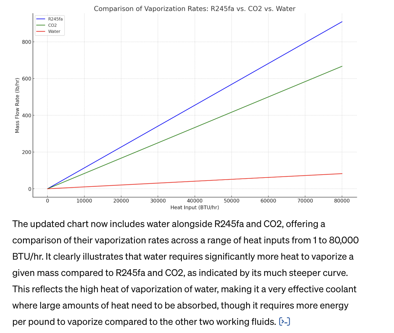
Now Compare Water

To include water in the comparison chart alongside R245fa and CO2, we need to consider the heat of vaporization for water. The heat of vaporization for water at its boiling point (100°C or 212°F) is approximately 970 BTU/lb. This value is much higher than those for R245fa and CO2, indicating that a significantly larger amount of energy is required to vaporize a pound of water.

Let's proceed to calculate the mass flow rate of water vaporized across the same range of heat inputs and update the chart to include water for a comprehensive comparison.

The updated chart now includes water alongside R245fa and CO2, offering a comparison of their vaporization rates across a range of heat inputs from 1 to 80,000 BTU/hr. It clearly illustrates that water requires significantly more heat to vaporize a given mass compared to R245fa and CO2, as indicated by its much steeper curve. This reflects the high heat of vaporization of water, making it a very effective coolant where large amounts of heat need to be absorbed, though it requires more energy per pound to vaporize compared to the other two working fluids.

CONTACT TEL: 608-238-6001 Email: greg@infinityturbine.com | RSS | AMP | PDF | IG | X.com